Predicting Heart Disease Risk with Random Forest

The goal of this project was to predict if a patient present heart disease based on test results, gender and age. The dataset is part of the UCI machine learning dataset.

Photo by Markus Frieauff

Methods

The analysis was performed using R. The dataset was cleaned according to the information gathered on the Kaggle discussion board. I used a decision tree and random Forest algorithms to identify patients with heart disease.

Load libraries

library(tidyverse)  # For data cleaning, sorting, and visualisation
library(DataExplorer) # For Exploratory Data Analysis
library(gridExtra) # To plot several plots in one figure
library(ggpubr) # To prepare publication-ready plots
library(GGally) # For correlations
library(caTools) # For classification model
library(rpart) # For classification model
library(rattle) # Plot nicer decision trees
library(randomForest) # For Random Forest model

I Data

heart-disease-uci Kaggle: https://www.kaggle.com/ronitf/heart-disease-uci

Useful links for this dataset

https://lucdemortier.github.io/projects/3_mcnulty

https://www.kaggle.com/ronitf/heart-disease-uci/discussion/105877

https://www.kaggle.com/ronitf/heart-disease-uci/discussion/93372

As explained on the links above, it is essential to note that on this dataset, the target value 0 indicates that the patient has heart disease.

Attribute Information:

age: age in years

sex: (1 = male; 0 = female)

cp: chest pain type (typical angina, atypical angina, non-angina, or asymptomatic angina)

trestbps: resting blood pressure (in mm Hg on admission to the hospital)

chol: serum cholestoral in mg/dl

fbs: Fasting blood sugar (< 120 mg/dl or > 120 mg/dl) (1 = true; 0 = false)

restecg: resting electrocardiographic results (normal, ST-T wave abnormality, or left ventricular hypertrophy)

thalach: Max. heart rate achieved during thalium stress test

exang: Exercise induced angina (1 = yes; 0 = no)

oldpeak: ST depression induced by exercise relative to rest

slope: Slope of peak exercise ST segment (0 = upsloping, 1 = flat, or 2 = downsloping)

ca: number of major vessels (0-3) colored by flourosopy 4 = NA

thal: Thalium stress test result 3 = normal; 6 = fixed defect; 7 = reversable defect 0 = NA

target: Heart disease status 1 or 0 (0 = heart disease 1 = asymptomatic)

df <- read_csv("./Data/heart.csv") # To read file on Kaggle

II Tidy dataset

copy <- df

df2 <- df %>%
  filter(
    thal != 0 & ca != 4 # remove values correspondind to NA in original dataset
  ) %>%
# Recode the categorical variables as factors using the dplyr library.
  mutate(
    sex = case_when(
      sex == 0 ~ "female",
      sex == 1 ~ "male"
           ),
    fbs = case_when(
      fbs == 0 ~ "<=120",
      fbs == 1 ~ ">120"
            ),
    exang = case_when(
      exang == 0 ~ "no",
      exang == 1 ~ "yes"
            ),
    cp = case_when(
      cp == 3 ~ "typical angina",
      cp == 1 ~ "atypical angina",
      cp == 2 ~ "non-anginal",
      cp == 0 ~ "asymptomatic angina"
          ),
    restecg = case_when(
      restecg == 0 ~ "hypertrophy",
      restecg == 1 ~ "normal",
      restecg == 2 ~ "wave abnormality"
              ),
    target = case_when(
      target == 1 ~ "asymptomatic",
      target == 0 ~ "heart-disease"
              ),
    slope = case_when(
      slope == 2 ~ "upsloping",
      slope == 1 ~ "flat",
      slope == 0 ~ "downsloping"
    ),
    thal = case_when(
      thal == 1 ~ "fixed defect",
      thal == 2 ~ "normal",
      thal == 3 ~ "reversable defect"
    ),
    sex = as.factor(sex),
    fbs = as.factor(fbs),
    exang = as.factor(exang),
    cp = as.factor(cp),
    slope = as.factor(slope),
    ca = as.factor(ca),
    thal = as.factor(thal)
  )
glimpse(df2) # Check that the transformation worked
plot_missing(df2) # Check that the transformation did not induce NA values

df <- df2 # Replace the df dataset by the tidy dataset

III Exploratory Data Analysis

A Visualise the data summary and distribution of each variable

df %>%
  summary()

##       age            sex                        cp         trestbps    
##  Min.   :29.00   female: 95   asymptomatic angina:141   Min.   : 94.0  
##  1st Qu.:48.00   male  :201   atypical angina    : 49   1st Qu.:120.0  
##  Median :56.00                non-anginal        : 83   Median :130.0  
##  Mean   :54.52                typical angina     : 23   Mean   :131.6  
##  3rd Qu.:61.00                                          3rd Qu.:140.0  
##  Max.   :77.00                                          Max.   :200.0  
##       chol          fbs        restecg             thalach      exang    
##  Min.   :126.0   <=120:253   Length:296         Min.   : 71.0   no :199  
##  1st Qu.:211.0   >120 : 43   Class :character   1st Qu.:133.0   yes: 97  
##  Median :242.5               Mode  :character   Median :152.5            
##  Mean   :247.2                                  Mean   :149.6            
##  3rd Qu.:275.2                                  3rd Qu.:166.0            
##  Max.   :564.0                                  Max.   :202.0            
##     oldpeak              slope     ca                     thal    
##  Min.   :0.000   downsloping: 21   0:173   fixed defect     : 18  
##  1st Qu.:0.000   flat       :137   1: 65   normal           :163  
##  Median :0.800   upsloping  :138   2: 38   reversable defect:115  
##  Mean   :1.059                     3: 20                          
##  3rd Qu.:1.650                                                    
##  Max.   :6.200                                                    
##     target         
##  Length:296        
##  Class :character  
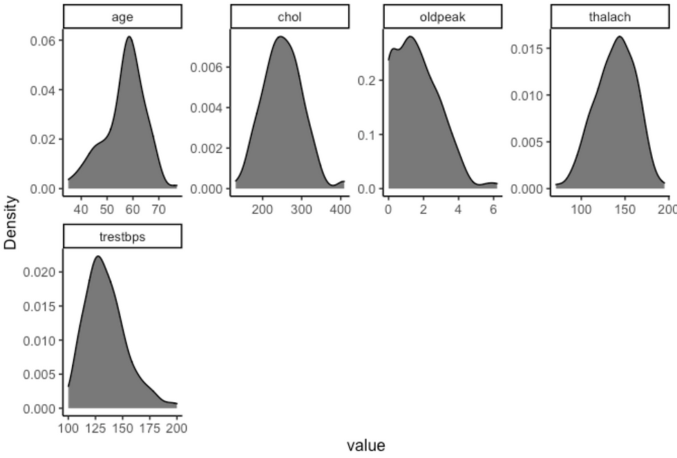
##  Mode  :character 

Use the DataExplorer library to get a sense of the distribution of the continuous and categorical variables.

plot_density(df, ggtheme = theme_classic2(), geom_density_args = list("fill" = "black", "alpha" = 0.6))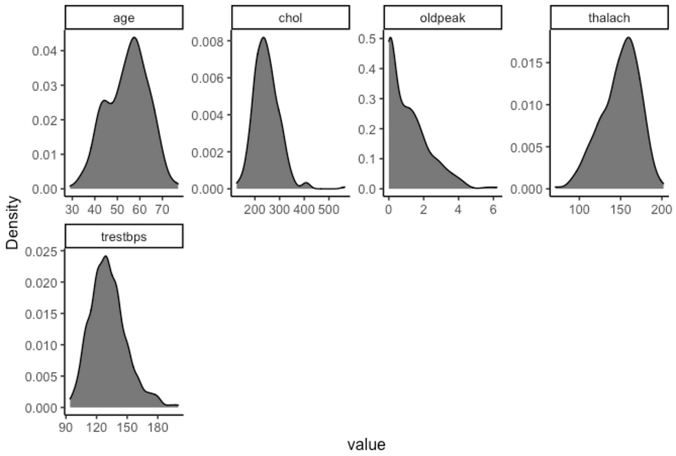

plot_bar(df, ggtheme = theme_classic2())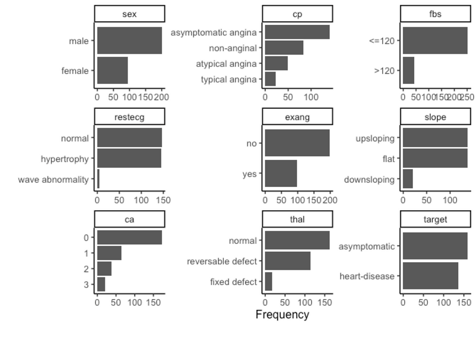

The next step is to combine dplyr and Data Explorer libraries to visualize the variables according to gender and disease.

B Analyse each variable per gender

df %>%
  filter(sex == "female") %>%
  plot_density(ggtheme = theme_classic2(), geom_density_args = list("fill" = "black", "alpha" = 0.6))

df %>%
  filter(sex == "male") %>%
  plot_density(ggtheme = theme_classic2(), geom_density_args = list("fill" = "black", "alpha" = 0.6))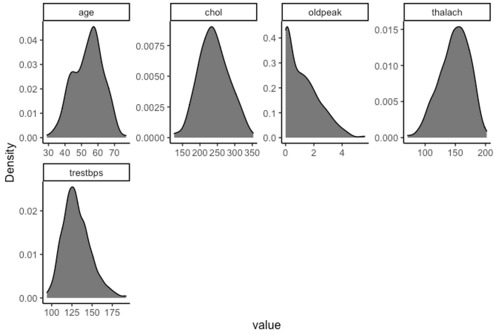

df %>%
  filter(sex == "female") %>%
  plot_bar(ggtheme = theme_classic2())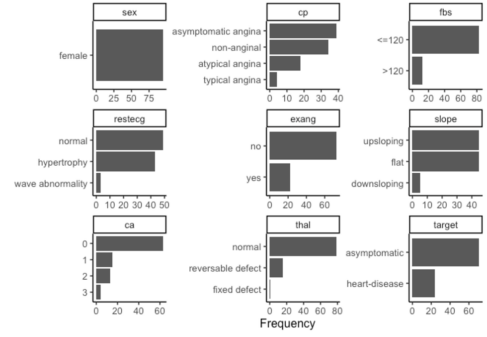

df %>%
  filter(sex == "male") %>%
  plot_bar(ggtheme = theme_classic2())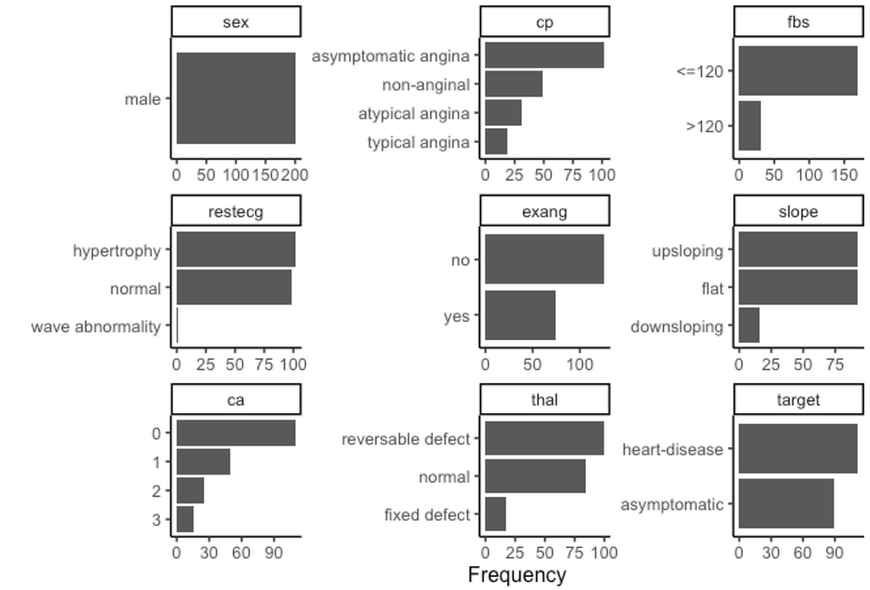

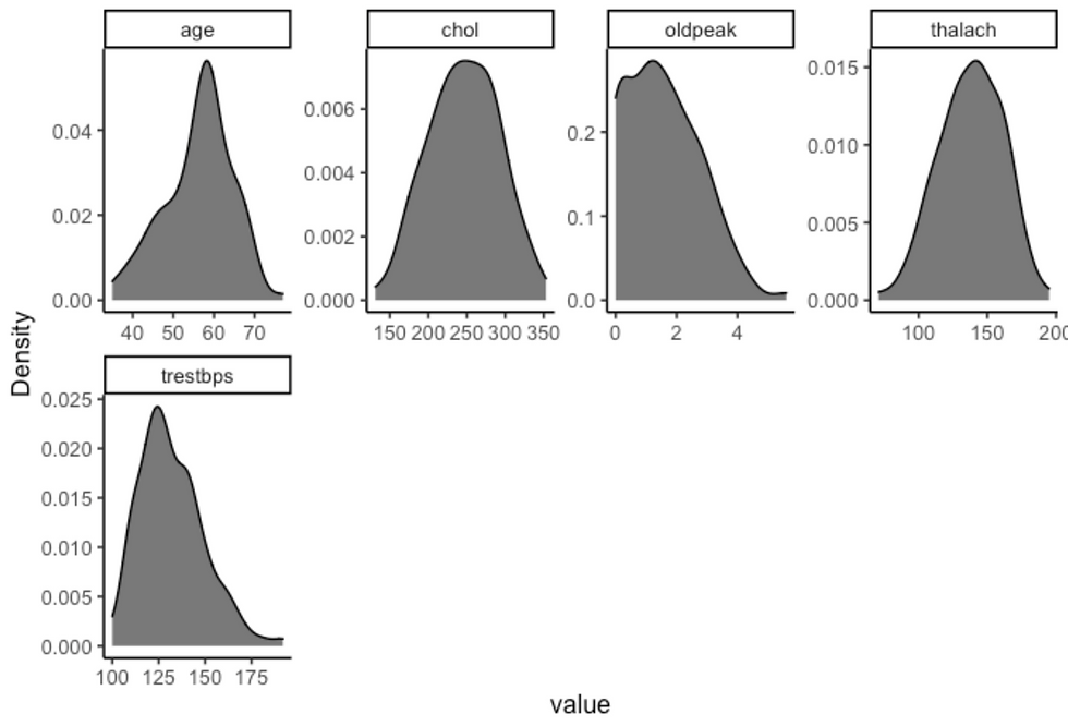
C Visualise variables per disease status

df %>%
  filter(target == "asymptomatic") %>%
  plot_density(ggtheme = theme_classic2(), geom_density_args = list("fill" = "black", "alpha" = 0.6))

df %>%
  filter(target == "heart-disease") %>%
  plot_density(ggtheme = theme_classic2(), geom_density_args = list("fill" = "black", "alpha" = 0.6))

df %>%
  filter(target == "asymptomatic") %>%
  plot_bar(ggtheme = theme_classic2())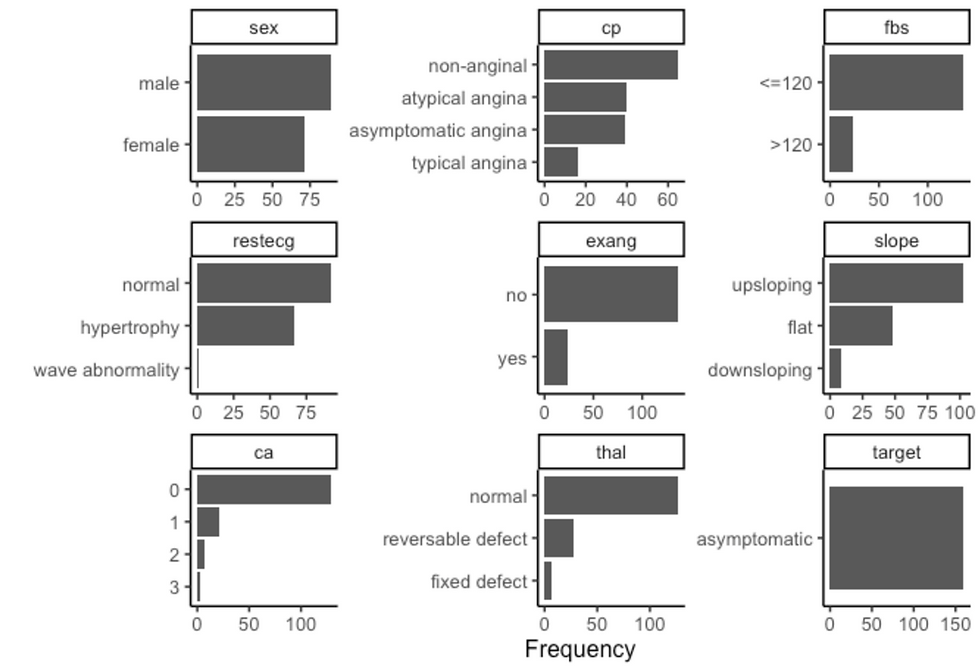

df %>%
  filter(target == "heart-disease") %>%
  plot_bar(ggtheme = theme_classic2())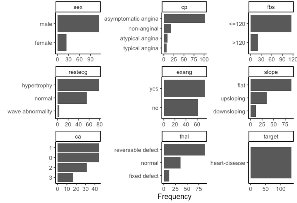

D Visualise the data per gender and disease status

df %>%
  filter(sex == "female", target == "asymptomatic") %>%
  plot_density(ggtheme = theme_classic2(), geom_density_args = list("fill" = "black", "alpha" = 0.6))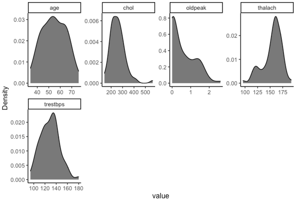

df %>%
  filter(sex == "female", target == "heart-disease") %>%
  plot_density(ggtheme = theme_classic2(), geom_density_args = list("fill" = "black", "alpha" = 0.6))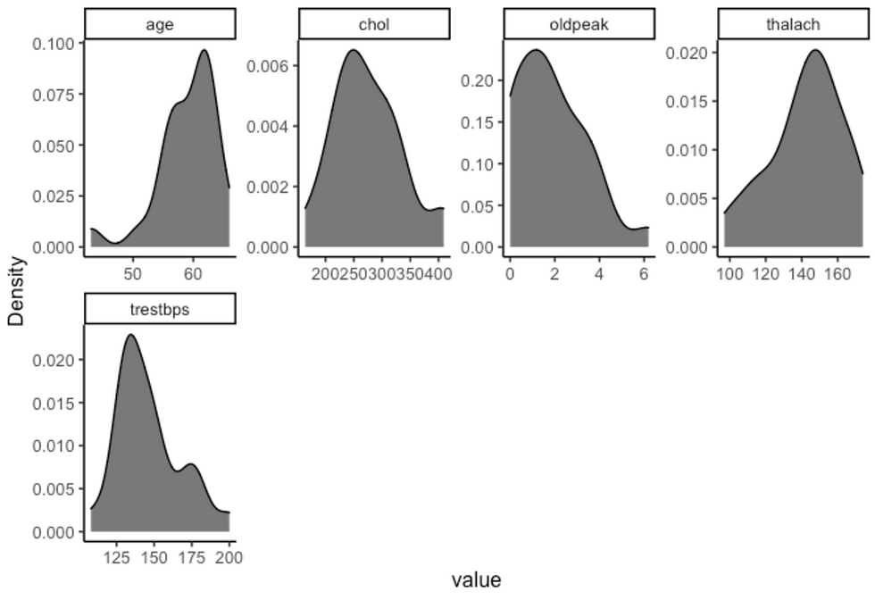

df %>%
  filter(sex == "female", target == "asymptomatic") %>%
  plot_bar(ggtheme = theme_classic2())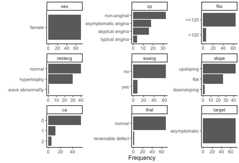

df %>%
  filter(sex == "female", target == "heart-disease") %>%
  plot_bar(ggtheme = theme_classic2())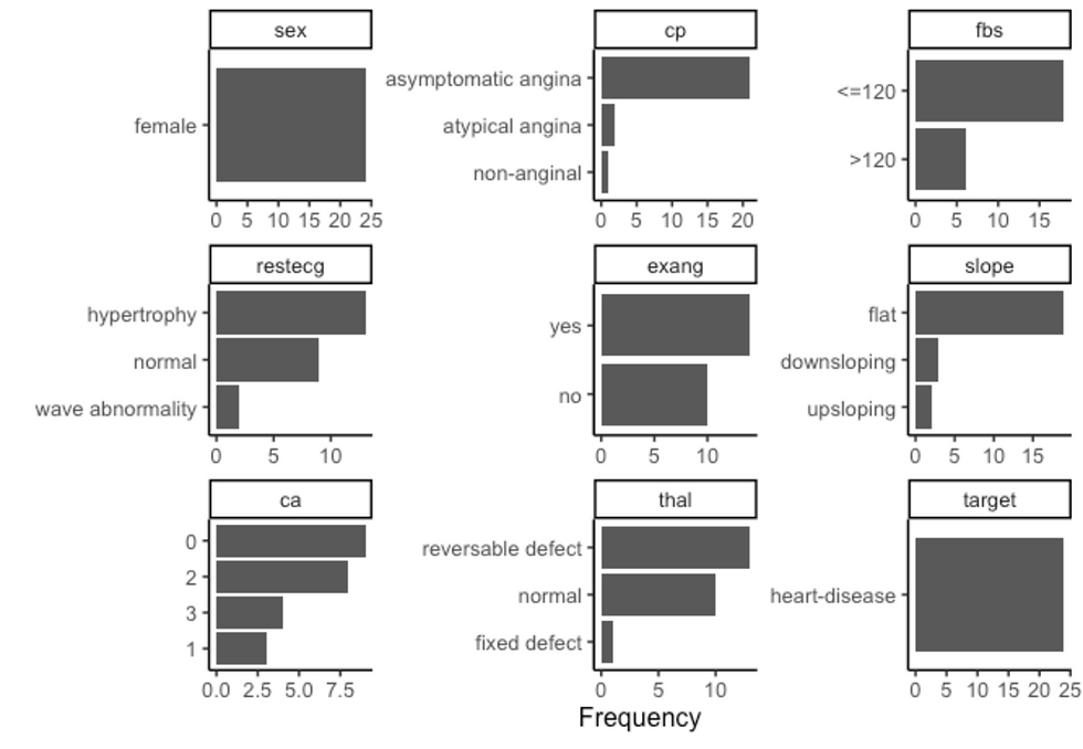

df %>%
  filter(sex == "male", target == "asymptomatic") %>%
  plot_density(ggtheme = theme_classic2(), geom_density_args = list("fill" = "black", "alpha" = 0.6))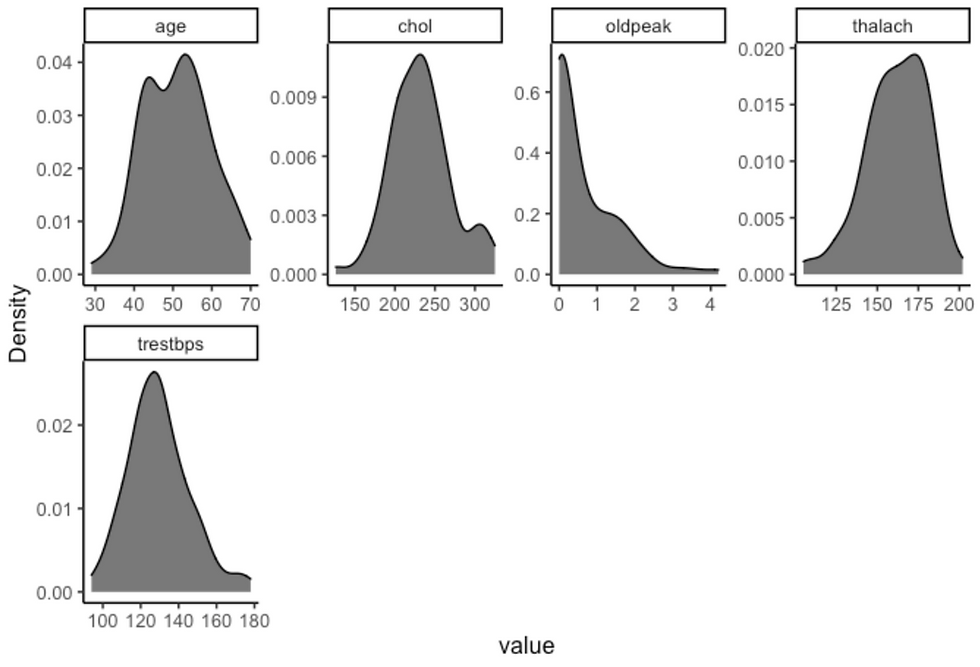

df %>%
  filter(sex == "male", target == "heart-disease") %>%
  plot_density(ggtheme = theme_classic2(), geom_density_args = list("fill" = "black", "alpha" = 0.6))

df %>%
  filter(sex == "male", target == "asymptomatic") %>%
  plot_bar(ggtheme = theme_classic2())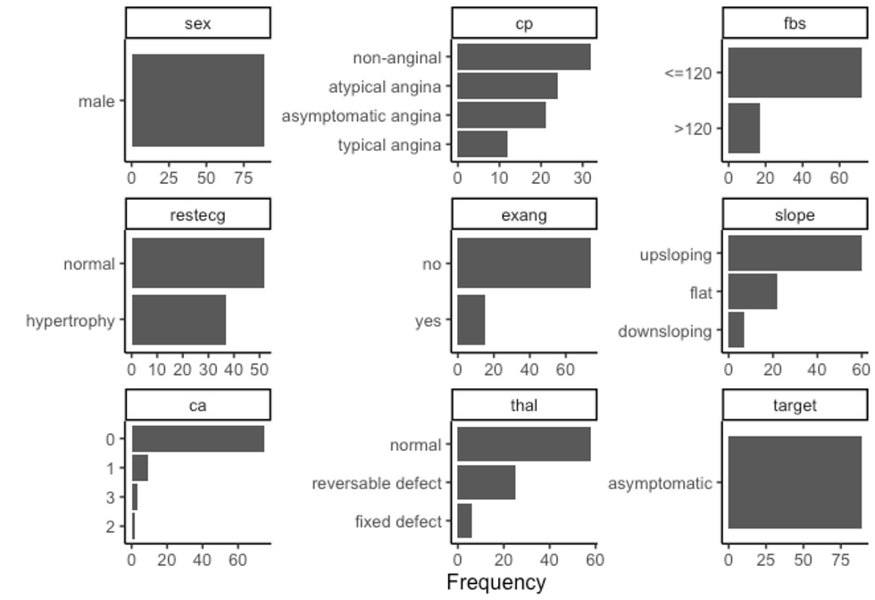

df %>%
  filter(sex == "male", target == "heart-disease") %>%
  plot_bar(ggtheme = theme_classic2())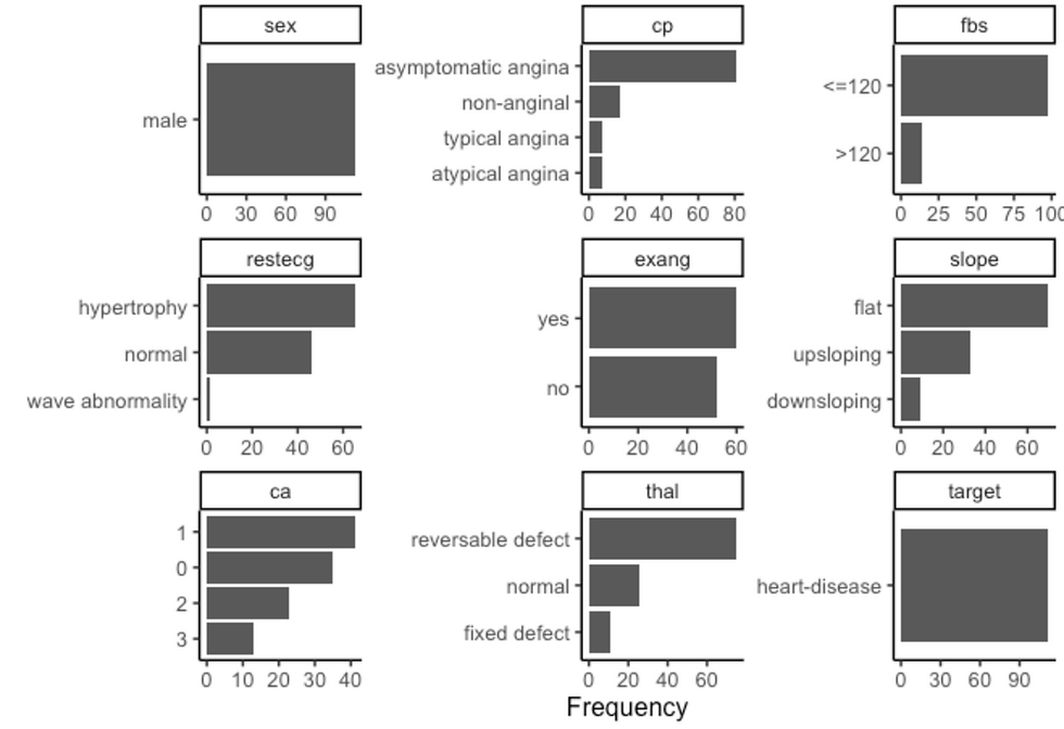

E Prepare a summary table per disease and gender

df %>%
  group_by(target, sex) %>%
  summarise(
    n_disease = n(),
    mean_age = round(mean(age), digits=2),
    sd_age = round(sd(age), digits=2),
    mean_trestbps = round(mean(trestbps), digits=2),
    sd_trestbps = round(sd(trestbps), digits=2),
    mean_chol = round(mean(chol), digits=2),
    sd_chol = round(sd(chol), digits=2),
    mean_thalach = round(mean(thalach), digits=2),
    sd_thalach = round(sd(thalach), digits=2),
    mean_oldpeak = round(mean(oldpeak), digits=2),
    sd_oldpeak = round(sd(oldpeak), digits=2)
  )

## `summarise()` has grouped output by 'target'. You can override using the `.groups` argument.

## # A tibble: 4 x 13
## # Groups:   target [2]
##   target sex   n_disease mean_age sd_age mean_trestbps sd_trestbps mean_chol
##   <chr>  <fct>     <int>    <dbl>  <dbl>         <dbl>       <dbl>     <dbl>
## 1 asymp… fema…        71     54.6  10.3           129.        16.6      257.
## 2 asymp… male         89     51.1   8.63          130.        16.2      232.
## 3 heart… fema…        24     59.0   4.96          146.        21.4      275.
## 4 heart… male        112     56.2   8.36          132.        17.4      246.
## # … with 5 more variables: sd_chol <dbl>, mean_thalach <dbl>, sd_thalach <dbl>,
## #   mean_oldpeak <dbl>, sd_oldpeak <dbl>

IV Data Visualisation

From the Exploratory Data analysis, it seems that several differences are statistically significant according to gender and health status.

A Visualisation of variables per gender

# Male and Female count
a1 <- ggplot(df, aes(x = sex, fill = sex)) +
  geom_bar(width = 0.5) + 
  scale_fill_manual(values = c("#386cb0","#fdb462"))+
  theme_classic2() +
  theme(legend.position='none')

# Age per gender
b1 <- ggplot(df, aes(x= sex, y = age, fill = sex)) +
  geom_violin(width = 0.5) +
  geom_boxplot(width = 0.2) +
  ylim(0, 90) +
  stat_compare_means(aes(label = ..p.signif..), method = "t.test") +
  scale_fill_manual(values = c("#386cb0","#fdb462"))+
  theme_classic2() +
  theme(legend.position='none')

# trestbps
c1 <- ggplot(df, aes(x = sex, y = trestbps, fill = sex)) +
  geom_violin(width = 0.5) +
  geom_boxplot(width = 0.2) + 
  labs(y = "blood pressure (mmHg)") +
  ylim(0,250) +
  stat_compare_means(aes(label = ..p.signif..), method = "t.test") +
  scale_fill_manual(values = c("#386cb0","#fdb462"))+
  theme_classic2() +
  theme(legend.position='none')

# chol
d1 <- ggplot(df, aes(x = sex, y = chol, fill = sex)) +
  geom_violin(width = 0.5) +
  geom_boxplot(width = 0.2) + 
  labs(y = "cholestorol (mg/dl)") +
  ylim(0,500) +
  stat_compare_means(aes(label = ..p.signif..), method = "t.test") +
  scale_fill_manual(values = c("#386cb0","#fdb462"))+
  theme_classic2() +
  theme(legend.position='none')

# oldpeak
e1 <- ggplot(df, aes(x = sex, y = oldpeak, fill = sex)) +
  geom_violin(width = 0.5) +
  geom_boxplot(width = 0.2) + 
  labs(y = "ST depression") +
  ylim(0,10) +
  stat_compare_means(aes(label = ..p.signif..), method = "t.test") +
  scale_fill_manual(values = c("#386cb0","#fdb462"))+
  theme_classic2() +
  theme(legend.position='none')

# thalach
f1 <- ggplot(df, aes(x = sex, y = thalach, fill = sex)) +
  geom_violin(width = 0.5) +
  geom_boxplot(width = 0.2) + 
  labs(y = "Max. heart rate") +
  ylim(0,250) +
  stat_compare_means(aes(label = ..p.signif..), method = "t.test") +
  scale_fill_manual(values = c("#386cb0","#fdb462"))+
  theme_classic2() +
  theme(legend.position='none')

suppressWarnings(ggarrange(a1, b1, c1, d1, e1, f1, 
          ncol = 2, nrow = 3,
            align = "v"))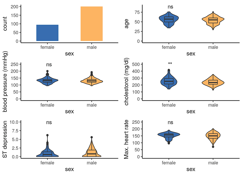

# Disease status
g1 <- ggplot(df, aes(x = target, fill = sex)) +
  geom_bar(width = 0.5, position = 'dodge') + 
  labs(x = "") +
  coord_flip() +
  scale_fill_manual(values = c("#386cb0","#fdb462"))+
  theme_classic2() +
  theme(legend.position='none')

# cp
h1 <- ggplot(df, aes(cp, group = sex, fill = sex)) +
  geom_bar(position = "dodge") +
  labs(x = "", y = "chest pain") +
  coord_flip() +
  scale_fill_manual(values = c("#386cb0","#fdb462"))+
  theme_classic2() +
  theme(legend.position='none')

# restecg
i1 <- ggplot(df, aes(restecg, group = sex, fill = sex)) +
  geom_bar(position = "dodge") +
  labs(x = "", y = "rest. electrocardiographic") +
  coord_flip() +
  scale_fill_manual(values = c("#386cb0","#fdb462"))+
  theme_classic2() +
  theme(legend.position='none')

# slope
j1 <- ggplot(df, aes(slope, group = sex, fill = sex)) +
  geom_bar(position = "dodge") +
  labs(x = "", y = "peak exercise ST") +
  coord_flip() +
  scale_fill_manual(values = c("#386cb0","#fdb462"))+
  theme_classic2() +
  theme(legend.position='none')

# thal 
k1 <- ggplot(df, aes(thal, group = sex, fill = sex)) +
  geom_bar(position = "dodge") +
  labs(x = "", y = "Thalium stress test") +
  coord_flip() +
  scale_fill_manual(values = c("#386cb0","#fdb462"))+
  theme_classic2() +
  theme(legend.position='none')

# fbp
l1 <- ggplot(df, aes(fbs, group = sex, fill = sex)) +
  geom_bar(position = "dodge") +
  labs(x = "", y = "Fasting blood sugar") +
  coord_flip() +
  scale_fill_manual(values = c("#386cb0","#fdb462"))+
  theme_classic2() +
  theme(legend.position='none')

# exang
m1 <- ggplot(df, aes(exang, group = sex, fill = sex)) +
  geom_bar(position = "dodge") +
  labs(x = "", y = "Exercise induced angina") +
  coord_flip() +
  scale_fill_manual(values = c("#386cb0","#fdb462"))+
  theme_classic2() +
  theme(legend.position='none')

# ca
n1 <- ggplot(df, aes(ca, group = sex, fill = sex)) +
  geom_bar(position = "dodge") +
  labs(x = "", y = "flourosopy") +
  coord_flip() +
  scale_fill_manual(values = c("#386cb0","#fdb462"))+
  theme_classic2() +
  theme(legend.position='none')

ggarrange(g1, h1, i1, j1, k1, l1, m1, n1, 
          ncol = 2, nrow = 4,
          align = "v")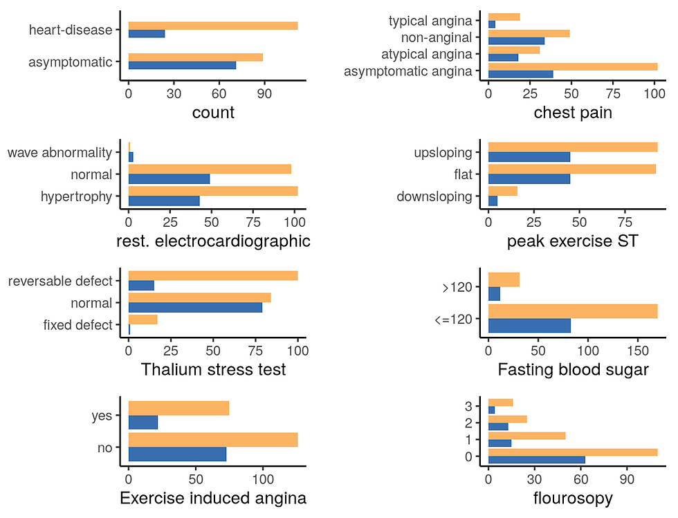

From this first plot, it appears that this dataset contains more males patients with a higher proportion of heart disease compared to female patients.

B Visualisation of variables per disease status

1 Male patient

df <- df2 %>%
    filter(sex == "male")

# Male and Female count
a2 <- ggplot(df, aes(x = target, fill = target)) +
  geom_bar(width = 0.5, position = 'dodge') + 
  scale_fill_manual(values = c("#7fc97f","#ef3b2c"))+
  theme_classic2() +
  theme(legend.position='none')

# Age per gender
b2 <- ggplot(df, aes(x= target, y = age, fill = target)) +
  geom_violin(width = 0.5) +
  geom_boxplot(width = 0.2) +
  ylim(0, 90) +
  stat_compare_means(aes(label = ..p.signif..), method = "t.test") +
  scale_fill_manual(values = c("#7fc97f","#ef3b2c"))+
  theme_classic2() +
  theme(legend.position='none')

# trestbps
c2 <- ggplot(df, aes(x = target, y = trestbps, fill = target)) +
  geom_violin(width = 0.5) +
  geom_boxplot(width = 0.2) + 
  labs(y = "blood pressure (mmHg)") +
  ylim(0,250) +
 stat_compare_means(aes(label = ..p.signif..), method = "t.test") +
  scale_fill_manual(values = c("#7fc97f","#ef3b2c"))+
  theme_classic2() +
  theme(legend.position='none')

# chol
d2 <- ggplot(df, aes(x = target, y = chol, fill = target)) +
  geom_violin(width = 0.5) +
  geom_boxplot(width = 0.2) + 
  labs(y = "cholestorol (mg/dl)") +
  ylim(0,500) +
  stat_compare_means(aes(label = ..p.signif..), method = "t.test") +
  scale_fill_manual(values = c("#7fc97f","#ef3b2c"))+
  theme_classic2() +
  theme(legend.position='none')

# oldpeak
e2 <- ggplot(df, aes(x = target, y = oldpeak, fill = target)) +
  geom_violin(width = 0.5) +
  geom_boxplot(width = 0.2) + 
  labs(y = "ST depression") +
  ylim(0,10) +
  stat_compare_means(aes(label = ..p.signif..), method = "t.test") +
  scale_fill_manual(values = c("#7fc97f","#ef3b2c"))+
  theme_classic2() +
  theme(legend.position='none')

# thalach
f2 <- ggplot(df, aes(x = target, y = thalach, fill = target)) +
  geom_violin(width = 0.5) +
  geom_boxplot(width = 0.2) + 
  labs(y = "Max. heart rate") +
  ylim(0,250) +
  stat_compare_means(aes(label = ..p.signif..), method = "t.test") +
  scale_fill_manual(values = c("#7fc97f","#ef3b2c"))+
  theme_classic2() +
  theme(legend.position='none')

ggarrange(a2, b2, c2, d2, e2, f2, 
          ncol = 2, nrow = 3,
            align = "v")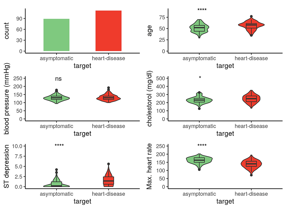

Male patients with heart disease are significantly older, have higher cholesterol level, and reduced maximum heart rate response to the thallium test.

# Disease status
g2 <- ggplot(df, aes(x = target, fill = target)) +
  geom_bar(width = 0.5, position = 'dodge') + 
  labs(x = "") +
  coord_flip() +
  scale_fill_manual(values = c("#7fc97f","#ef3b2c"))+
  theme_classic2() +
  theme(legend.position='none')

# cp
h2 <- ggplot(df, aes(cp, group = target, fill = target)) +
  geom_bar(position = "dodge") +
  labs(x = "", y = "chest pain") +
  coord_flip() +
  scale_fill_manual(values = c("#7fc97f","#ef3b2c"))+
  theme_classic2() +
  theme(legend.position='none')

# restecg
i2 <- ggplot(df, aes(restecg, group = target, fill = target)) +
  geom_bar(position = "dodge") +
  labs(x = "", y = "rest. electrocardiographic") +
  coord_flip() +
  scale_fill_manual(values = c("#7fc97f","#ef3b2c"))+
  theme_classic2() +
  theme(legend.position='none')

# slope
j2 <- ggplot(df, aes(slope, group = target, fill = target)) +
  geom_bar(position = "dodge") +
  labs(x = "", y = "peak exercise ST") +
  coord_flip() +
  scale_fill_manual(values = c("#7fc97f","#ef3b2c"))+
  theme_classic2() +
  theme(legend.position='none')

# thal 
k2 <- ggplot(df, aes(thal, group = target, fill = target)) +
  geom_bar(position = "dodge") +
  labs(x = "", y = "Thalium stress test") +
  coord_flip() +
  scale_fill_manual(values = c("#7fc97f","#ef3b2c"))+
  theme_classic2() +
  theme(legend.position='none')

# fbp
l2 <- ggplot(df, aes(fbs, group = target, fill = target)) +
  geom_bar(position = "dodge") +
  labs(x = "", y = "Fasting blood sugar") +
  coord_flip() +
  scale_fill_manual(values = c("#7fc97f","#ef3b2c"))+
  theme_classic2() +
  theme(legend.position='none')

# exang
m2 <- ggplot(df, aes(exang, group = target, fill = target)) +
  geom_bar(position = "dodge") +
  labs(x = "", y = "Exercise induced angina") +
  coord_flip() +
  scale_fill_manual(values = c("#7fc97f","#ef3b2c"))+
  theme_classic2() +
  theme(legend.position='none')

# ca
n2 <- ggplot(df, aes(ca, group = target, fill = target)) +
  geom_bar(position = "dodge") +
  labs(x = "", y = "flourosopy") +
  coord_flip() +
  scale_fill_manual(values = c("#7fc97f","#ef3b2c"))+
  theme_classic2() +
  theme(legend.position='none')

ggarrange(g2, h2, i2, j2, k2, l2, m2, n2, 
          ncol = 2, nrow = 4,
          align = "v")

2 Female patients

df <- df2 %>%
    filter(sex == "female")

# Male and Female count
a2 <- ggplot(df, aes(x = target, fill = target)) +
  geom_bar(width = 0.5, position = 'dodge') + 
  scale_fill_manual(values = c("#7fc97f","#ef3b2c"))+
  theme_classic2() +
  theme(legend.position='none')

# Age per gender
b2 <- ggplot(df, aes(x= target, y = age, fill = target)) +
  geom_violin(width = 0.5) +
  geom_boxplot(width = 0.2) +
  ylim(0, 90) +
  stat_compare_means(aes(label = ..p.signif..), method = "t.test") +
  scale_fill_manual(values = c("#7fc97f","#ef3b2c"))+
  theme_classic2() +
  theme(legend.position='none')

# trestbps
c2 <- ggplot(df, aes(x = target, y = trestbps, fill = target)) +
  geom_violin(width = 0.5) +
  geom_boxplot(width = 0.2) + 
  labs(y = "blood pressure (mmHg)") +
  ylim(0,250) +
  stat_compare_means(aes(label = ..p.signif..), method = "t.test") +
  scale_fill_manual(values = c("#7fc97f","#ef3b2c"))+
  theme_classic2() +
  theme(legend.position='none')

# chol
d2 <- ggplot(df, aes(x = target, y = chol, fill = target)) +
  geom_violin(width = 0.5) +
  geom_boxplot(width = 0.2) + 
  labs(y = "cholestorol (mg/dl)") +
  ylim(0,500) +
  stat_compare_means(aes(label = ..p.signif..), method = "t.test") +
  scale_fill_manual(values = c("#7fc97f","#ef3b2c"))+
  theme_classic2() +
  theme(legend.position='none')

# oldpeak
e2 <- ggplot(df, aes(x = target, y = oldpeak, fill = target)) +
  geom_violin(width = 0.5) +
  geom_boxplot(width = 0.2) + 
  labs(y = "ST depression") +
  ylim(0,10) +
  stat_compare_means(aes(label = ..p.signif..), method = "t.test") +
  scale_fill_manual(values = c("#7fc97f","#ef3b2c"))+
  theme_classic2() +
  theme(legend.position='none')

# thalach
f2 <- ggplot(df, aes(x = target, y = thalach, fill = target)) +
  geom_violin(width = 0.5) +
  geom_boxplot(width = 0.2) + 
  labs(y = "Max. heart rate") +
  ylim(0,250) +
  stat_compare_means(aes(label = ..p.signif..), method = "t.test") +
  scale_fill_manual(values = c("#7fc97f","#ef3b2c"))+
  theme_classic2() +
  theme(legend.position='none')

suppressWarnings(ggarrange(a2, b2, c2, d2, e2, f2, 
          ncol = 2, nrow = 3,
            align = "v"))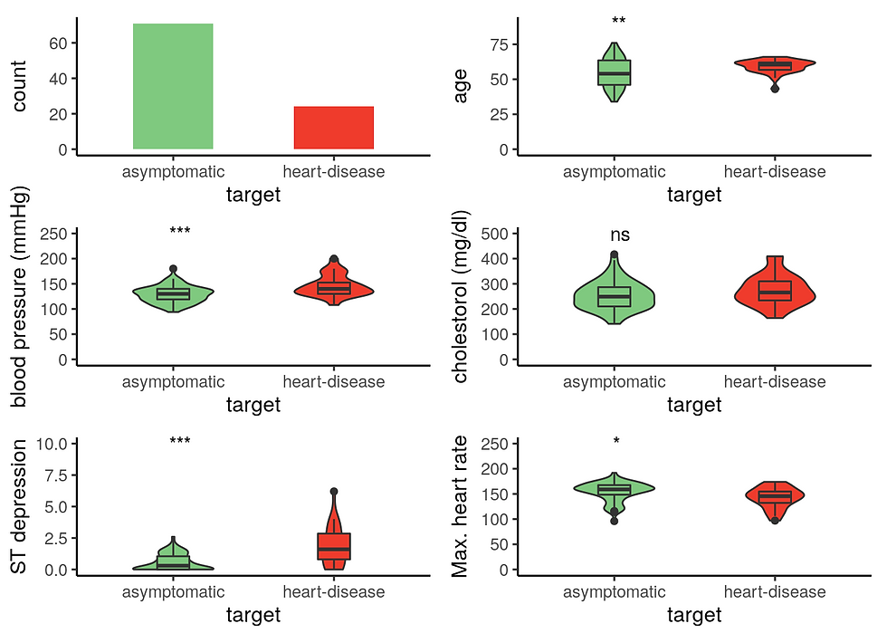

There is less woman with heart disease on this data set. Women with heart disease have a significantly higher resting blood presure contrary to male with heart disease. Similarly to men, women with heart disease have a lower maximum heart rate in response to the thallium test.

# Disease status
g2 <- ggplot(df, aes(x = target, fill = target)) +
  geom_bar(width = 0.5, position = 'dodge') + 
  labs(x = "") +
  coord_flip() +
  scale_fill_manual(values = c("#7fc97f","#ef3b2c"))+
  theme_classic2() +
  theme(legend.position='none')

# cp
h2 <- ggplot(df, aes(cp, group = target, fill = target)) +
  geom_bar(position = "dodge") +
  labs(x = "", y = "chest pain") +
  coord_flip() +
  scale_fill_manual(values = c("#7fc97f","#ef3b2c"))+
  theme_classic2() +
  theme(legend.position='none')

# restecg
i2 <- ggplot(df, aes(restecg, group = target, fill = target)) +
  geom_bar(position = "dodge") +
  labs(x = "", y = "rest. electrocardiographic") +
  coord_flip() +
  scale_fill_manual(values = c("#7fc97f","#ef3b2c"))+
  theme_classic2() +
  theme(legend.position='none')

# slope
j2 <- ggplot(df, aes(slope, group = target, fill = target)) +
  geom_bar(position = "dodge") +
  labs(x = "", y = "peak exercise ST") +
  coord_flip() +
  scale_fill_manual(values = c("#7fc97f","#ef3b2c"))+
  theme_classic2() +
  theme(legend.position='none')

# thal 
k2 <- ggplot(df, aes(thal, group = target, fill = target)) +
  geom_bar(position = "dodge") +
  labs(x = "", y = "Thalium stress test") +
  coord_flip() +
  scale_fill_manual(values = c("#7fc97f","#ef3b2c"))+
  theme_classic2() +
  theme(legend.position='none')

# fbp
l2 <- ggplot(df, aes(fbs, group = target, fill = target)) +
  geom_bar(position = "dodge") +
  labs(x = "", y = "Fasting blood sugar") +
  coord_flip() +
  scale_fill_manual(values = c("#7fc97f","#ef3b2c"))+
  theme_classic2() +
  theme(legend.position='none')

# exang
m2 <- ggplot(df, aes(exang, group = target, fill = target)) +
  geom_bar(position = "dodge") +
  labs(x = "", y = "Exercise induced angina") +
  coord_flip() +
  scale_fill_manual(values = c("#7fc97f","#ef3b2c"))+
  theme_classic2() +
  theme(legend.position='none')

# ca
n2 <- ggplot(df, aes(ca, group = target, fill = target)) +
  geom_bar(position = "dodge") +
  labs(x = "", y = "flourosopy") +
  coord_flip() +
  scale_fill_manual(values = c("#7fc97f","#ef3b2c"))+
  theme_classic2() +
  theme(legend.position='none')

ggarrange(g2, h2, i2, j2, k2, l2, m2, n2, 
          ncol = 2, nrow = 4,
          align = "v")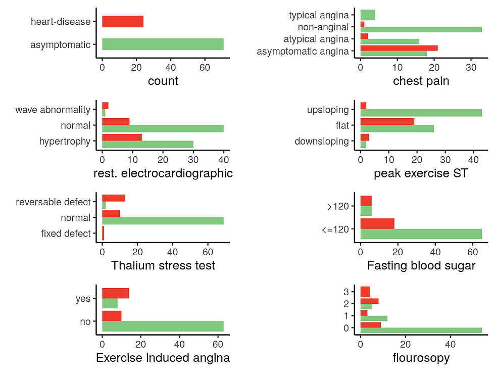

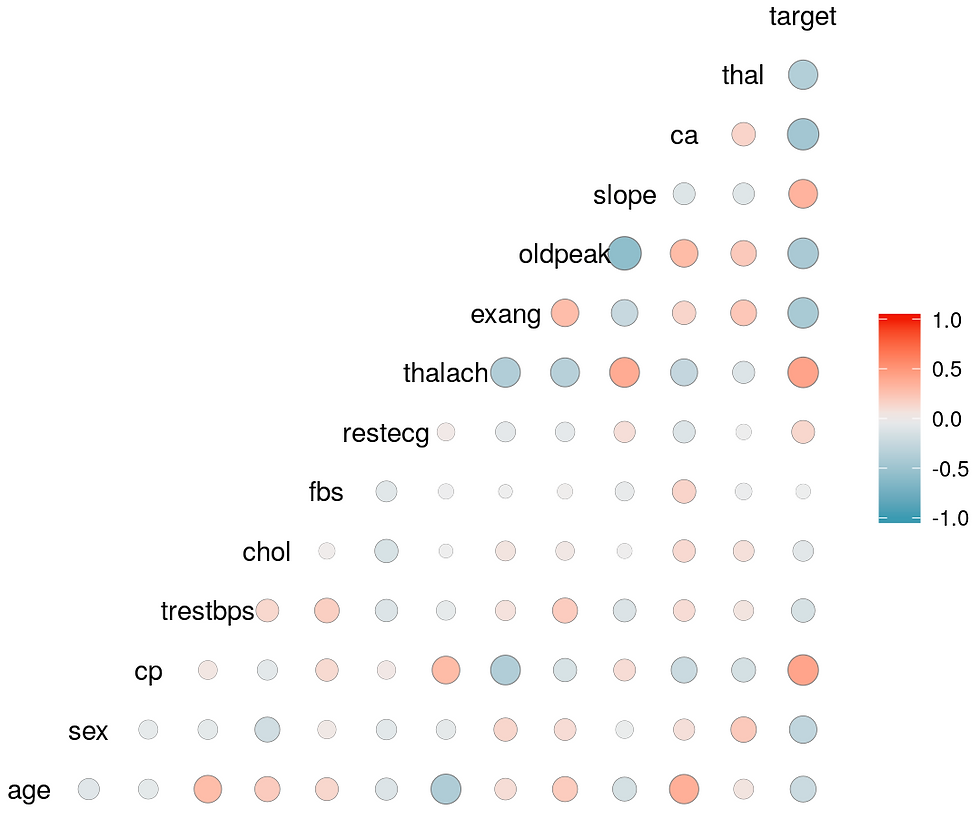
V Correlations

A use the numerical dataset

df <- copy %>%
  filter(
    thal != 0 & ca != 4 # remove values corresponding to NA in original dataset
    )

# ggcorr(df, palette = "RdBu")
GGally::ggcorr(df, geom = "circle")

select2 <- df %>%
  dplyr::select(
    target,
    slope,
    thalach,
    restecg,
    cp
  )
ggcorr(select2, geom = "circle")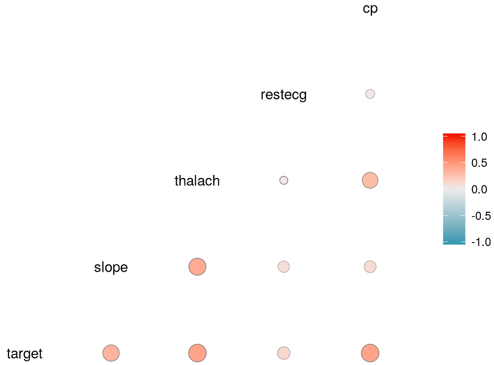

ggpairs(select2)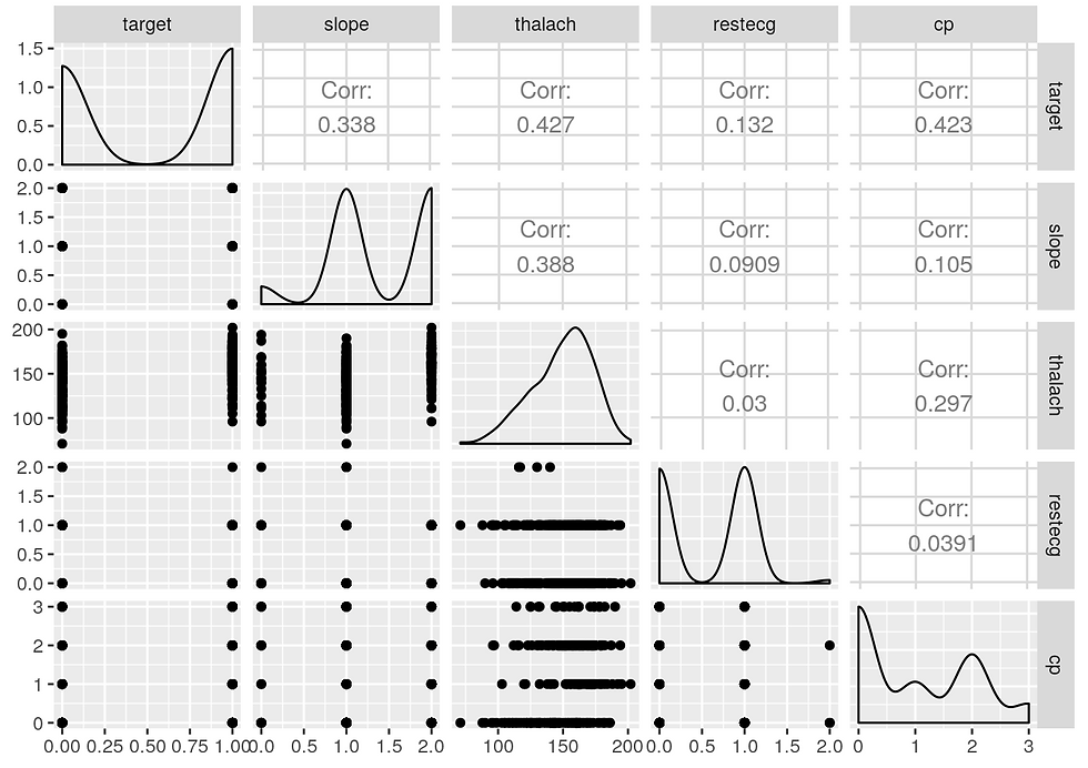

From the correlation study it seems that the parameters: cp, restecg, thalach, slope

are the most useful to predict the risk of heart disease

From the EDA analysis it seems that: age, sex, cholesterol, restecg

are also useful

For prediction the following variables seems the most useful: age, sex, cholesterol, restecg, cp, thalach, slope

VI Machine Learning: classification model with rpart and random forest packages

1. Select the columns useful for prediction according to the EDA analysis.

2. Separate the data set in a train and test subsets.

3. Build a classification tree model with rpart.

4. Print model accuracy and decision tree.

A Use select columns for classification

df_select <- df %>%
  dplyr::select( #because of conflict between MASS and dplyr select need to use dplyr::select
    target,
    age,
    sex,
    chol,
    restecg,
    cp,
    thalach,
    slope
  )

df_select$target <- factor(df_select$target) # Define target as a factor. rpart classification would not work otherwise.

accuracy <- 0

# Build a simple classification desicion tree with rpart. Run the model until the accuracy reach the selected minimum.
while(accuracy <= 0.85) {
  split_values <- sample.split(df_select$target, SplitRatio = 0.65)
  train_set <- subset(df_select, split_values == T)
  test_set <- subset(df_select, split_values == F)
  mod_class <- rpart(target~. , data=train_set)
  result_class <- predict(mod_class, test_set, type = "class")
  table <- table(test_set$target, result_class)
  accuracy <- (table["0","0"] + table["1","1"])/sum(table)
  # cat("accuracy = ", round(accuracy, digits = 2)*100, "%")
}

Print model accuracy.

According to this parameters the model should be at least 85% accurate.

cat("Model accuracy", round(accuracy, digits = 2)*100, "%") 

## Model accuracy 86 %

Print the decision tree.

# par(mfrow = c(1,2), xpd = NA) # otherwise on some devices the text is clipped
fancyRpartPlot(mod_class, , caption = NULL)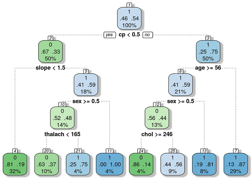

B Use the full dataset for classification

copy2 <- df
df$target <- factor(df$target)
accuracy <- 0

# Build a simple classification desicion tree with rpart. Run the model until the accuracy reach the selected minimum.
while(accuracy <= 0.88) {
  split_values <- sample.split(df_select$target, SplitRatio = 0.65)
  train_set <- subset(df, split_values == T)
  test_set <- subset(df, split_values == F)
  mod_class <- rpart(target~. , data=train_set)
  result_class <- predict(mod_class, test_set, type = "class")
  table <- table(test_set$target, result_class)
  accuracy <- (table["0","0"] + table["1","1"])/sum(table)
  # cat("accuracy = ", round(accuracy, digits = 2)*100, "%")
}

Print model accuracy.

According to the parameters the model should be at least 88% accurate.

cat("Model accuracy", round(accuracy, digits = 2)*100, "%")  

## Model accuracy 89 %

Print the decision tree.

# par(mfrow = c(1,2), xpd = NA) # otherwise on some devices the text is clipped
fancyRpartPlot(mod_class, , caption = NULL)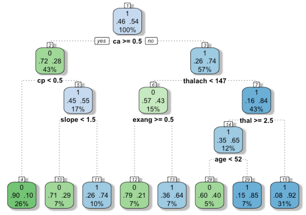

C Prediction on selected column with random forest

set.seed(123)
train <- sample(nrow(df_select), 0.7*nrow(df_select), replace = FALSE)
TrainSet <- df_select[train,]
ValidSet <- df_select[-train,]
summary(TrainSet)

##  target       age             sex              chol        restecg      
##  0: 91   Min.   :29.00   Min.   :0.0000   Min.   :126   Min.   :0.0000  
##  1:116   1st Qu.:48.00   1st Qu.:0.0000   1st Qu.:208   1st Qu.:0.0000  
##          Median :56.00   Median :1.0000   Median :240   Median :0.0000  
##          Mean   :55.02   Mean   :0.6763   Mean   :244   Mean   :0.5024  
##          3rd Qu.:62.00   3rd Qu.:1.0000   3rd Qu.:272   3rd Qu.:1.0000  
##          Max.   :77.00   Max.   :1.0000   Max.   :564   Max.   :2.0000  
##        cp           thalach          slope      
##  Min.   :0.000   Min.   : 95.0   Min.   :0.000  
##  1st Qu.:0.000   1st Qu.:136.0   1st Qu.:1.000  
##  Median :1.000   Median :153.0   Median :1.000  
##  Mean   :1.014   Mean   :150.2   Mean   :1.386  
##  3rd Qu.:2.000   3rd Qu.:165.0   3rd Qu.:2.000  
##  Max.   :3.000   Max.   :202.0   Max.   :2.000

summary(ValidSet)

##  target      age             sex              chol          restecg     
##  0:45   Min.   :35.00   Min.   :0.0000   Min.   :175.0   Min.   :0.000  
##  1:44   1st Qu.:47.00   1st Qu.:0.0000   1st Qu.:223.0   1st Qu.:0.000  
##         Median :54.00   Median :1.0000   Median :247.0   Median :1.000  
##         Mean   :53.37   Mean   :0.6854   Mean   :254.5   Mean   :0.573  
##         3rd Qu.:59.00   3rd Qu.:1.0000   3rd Qu.:283.0   3rd Qu.:1.000  
##         Max.   :70.00   Max.   :1.0000   Max.   :409.0   Max.   :2.000  
##        cp            thalach          slope      
##  Min.   :0.0000   Min.   : 71.0   Min.   :0.000  
##  1st Qu.:0.0000   1st Qu.:132.0   1st Qu.:1.000  
##  Median :0.0000   Median :152.0   Median :1.000  
##  Mean   :0.8315   Mean   :148.2   Mean   :1.416  
##  3rd Qu.:2.0000   3rd Qu.:168.0   3rd Qu.:2.000  
##  Max.   :3.0000   Max.   :190.0   Max.   :2.000

# Create a Random Forest model with default parameters
model1 <- randomForest(target ~ ., data = TrainSet,  ntree = 1000, mtry = 1, importance = TRUE)
model1

## 
## Call:
##  randomForest(formula = target ~ ., data = TrainSet, ntree = 1000,      mtry = 1, importance = TRUE) 
##                Type of random forest: classification
##                      Number of trees: 1000
## No. of variables tried at each split: 1
## 
##         OOB estimate of  error rate: 28.02%
## Confusion matrix:
##    0  1 class.error
## 0 58 33   0.3626374
## 1 25 91   0.2155172

# Predicting on Validation set
predValid <- predict(model1, ValidSet, type = "class")
# Checking classification accuracy
mean(predValid == ValidSet$target)           

## [1] 0.7977528

table(predValid,ValidSet$target)

##          
## predValid  0  1
##         0 36  9
##         1  9 35

# To check important variables
importance(model1) 

##                 0            1 MeanDecreaseAccuracy MeanDecreaseGini
## age      3.456978 11.118814352            10.045334        10.174882
## sex     17.986950 18.447097660            22.356657         6.212641
## chol    -3.667658 -0.005187581            -2.378170         9.368247
## restecg  1.926634  3.951377314             4.138125         3.080821
## cp      19.676722 17.420672992            22.537720        10.408636
## thalach 14.987882 12.899451821            18.350082        14.006896
## slope   13.982290  9.048798817            15.232708         6.022085

varImpPlot(model1)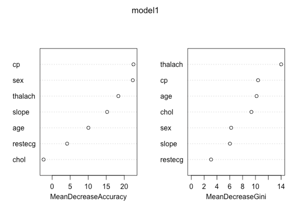  

D Use the full dataset for classification with random forest

set.seed(123)
train <- sample(nrow(df), 0.7*nrow(df_select), replace = FALSE)
TrainSet <- df[train,]
ValidSet <- df[-train,]
summary(TrainSet)

##       age             sex               cp           trestbps          chol    
##  Min.   :29.00   Min.   :0.0000   Min.   :0.000   Min.   :100.0   Min.   :126  
##  1st Qu.:48.00   1st Qu.:0.0000   1st Qu.:0.000   1st Qu.:120.0   1st Qu.:208  
##  Median :56.00   Median :1.0000   Median :1.000   Median :130.0   Median :240  
##  Mean   :55.02   Mean   :0.6763   Mean   :1.014   Mean   :131.1   Mean   :244  
##  3rd Qu.:62.00   3rd Qu.:1.0000   3rd Qu.:2.000   3rd Qu.:140.0   3rd Qu.:272  
##  Max.   :77.00   Max.   :1.0000   Max.   :3.000   Max.   :192.0   Max.   :564  
##       fbs            restecg          thalach          exang       
##  Min.   :0.0000   Min.   :0.0000   Min.   : 95.0   Min.   :0.0000  
##  1st Qu.:0.0000   1st Qu.:0.0000   1st Qu.:136.0   1st Qu.:0.0000  
##  Median :0.0000   Median :0.0000   Median :153.0   Median :0.0000  
##  Mean   :0.1643   Mean   :0.5024   Mean   :150.2   Mean   :0.3382  
##  3rd Qu.:0.0000   3rd Qu.:1.0000   3rd Qu.:165.0   3rd Qu.:1.0000  
##  Max.   :1.0000   Max.   :2.0000   Max.   :202.0   Max.   :1.0000  
##     oldpeak          slope             ca              thal       target 
##  Min.   :0.000   Min.   :0.000   Min.   :0.0000   Min.   :1.000   0: 91  
##  1st Qu.:0.000   1st Qu.:1.000   1st Qu.:0.0000   1st Qu.:2.000   1:116  
##  Median :0.800   Median :1.000   Median :0.0000   Median :2.000          
##  Mean   :1.055   Mean   :1.386   Mean   :0.6039   Mean   :2.319          
##  3rd Qu.:1.600   3rd Qu.:2.000   3rd Qu.:1.0000   3rd Qu.:3.000          
##  Max.   :6.200   Max.   :2.000   Max.   :3.0000   Max.   :3.000

summary(ValidSet)

##       age             sex               cp            trestbps    
##  Min.   :35.00   Min.   :0.0000   Min.   :0.0000   Min.   : 94.0  
##  1st Qu.:47.00   1st Qu.:0.0000   1st Qu.:0.0000   1st Qu.:120.0  
##  Median :54.00   Median :1.0000   Median :0.0000   Median :130.0  
##  Mean   :53.37   Mean   :0.6854   Mean   :0.8315   Mean   :132.8  
##  3rd Qu.:59.00   3rd Qu.:1.0000   3rd Qu.:2.0000   3rd Qu.:146.0  
##  Max.   :70.00   Max.   :1.0000   Max.   :3.0000   Max.   :200.0  
##       chol            fbs            restecg         thalach     
##  Min.   :175.0   Min.   :0.0000   Min.   :0.000   Min.   : 71.0  
##  1st Qu.:223.0   1st Qu.:0.0000   1st Qu.:0.000   1st Qu.:132.0  
##  Median :247.0   Median :0.0000   Median :1.000   Median :152.0  
##  Mean   :254.5   Mean   :0.1011   Mean   :0.573   Mean   :148.2  
##  3rd Qu.:283.0   3rd Qu.:0.0000   3rd Qu.:1.000   3rd Qu.:168.0  
##  Max.   :409.0   Max.   :1.0000   Max.   :2.000   Max.   :190.0  
##      exang           oldpeak          slope             ca        
##  Min.   :0.0000   Min.   :0.000   Min.   :0.000   Min.   :0.0000  
##  1st Qu.:0.0000   1st Qu.:0.000   1st Qu.:1.000   1st Qu.:0.0000  
##  Median :0.0000   Median :0.800   Median :1.000   Median :1.0000  
##  Mean   :0.3034   Mean   :1.069   Mean   :1.416   Mean   :0.8539  
##  3rd Qu.:1.0000   3rd Qu.:1.900   3rd Qu.:2.000   3rd Qu.:1.0000  
##  Max.   :1.0000   Max.   :4.400   Max.   :2.000   Max.   :3.0000  
##       thal       target
##  Min.   :1.000   0:45  
##  1st Qu.:2.000   1:44  
##  Median :2.000         
##  Mean   :2.348         
##  3rd Qu.:3.000         
##  Max.   :3.000

# Create a Random Forest model with default parameters
model2 <- randomForest(target ~ ., data = TrainSet,  ntree = 1000, mtry = 2, importance = TRUE)
model2

## 
## Call:
##  randomForest(formula = target ~ ., data = TrainSet, ntree = 1000,      mtry = 2, importance = TRUE) 
##                Type of random forest: classification
##                      Number of trees: 1000
## No. of variables tried at each split: 2
## 
##         OOB estimate of  error rate: 20.77%
## Confusion matrix:
##    0   1 class.error
## 0 63  28   0.3076923
## 1 15 101   0.1293103

# Predicting on train set
predTrain <- predict(model2, TrainSet, type = "class")
# Checking classification accuracy
table(predTrain, TrainSet$target)

##          
## predTrain   0   1
##         0  91   0
##         1   0 116

# Predicting on Validation set
predValid <- predict(model2, ValidSet, type = "class")
# Checking classification accuracy
mean(predValid == ValidSet$target)                    

## [1] 0.8764045

table(predValid,ValidSet$target)

##          
## predValid  0  1
##         0 39  5
##         1  6 39

# To check important variables
importance(model2)        

##                  0          1 MeanDecreaseAccuracy MeanDecreaseGini
## age       4.050036  6.7463054             7.778196         8.939681
## sex       8.638348 14.3957620            15.929672         4.589083
## cp       15.051396 11.2883097            17.483834         9.059950
## trestbps  1.813027  0.9226925             2.032148         7.050590
## chol     -1.726460 -2.4182808            -2.982013         8.319708
## fbs      -1.802818  4.1916949             2.098540         1.367634
## restecg   1.178421  2.2335381             2.450169         2.609878
## thalach   9.766391 10.4880323            14.128124        12.069991
## exang     9.185204  5.9611054            10.635688         4.988638
## oldpeak  18.583582 18.0805610            24.266457        12.847074
## slope     8.688542  4.0812821             9.073868         4.321699
## ca       22.053674 24.4175996            29.812574        11.204931
## thal     14.724654 16.1138529            19.564541         8.636882

varImpPlot(model2)

References

Data transformation

• https://archive.ics.uci.edu/ml/datasets/Heart+Disease

• https://lucdemortier.github.io/projects/3_mcnulty

• https://www.kaggle.com/ronitf/heart-disease-uci/discussion/105877

Kaggles notebooks:

• https://www.kaggle.com/ekrembayar/heart-disease-uci-eda-models-with-r

• https://www.kaggle.com/joemenifee/heart-disease-uci-data-exploratory

Data Processing

• http://www.cookbook-r.com/

• https://bookdown.org/rdpeng/exdata/managing-data-frames-with-the-dplyr-package.html#data-frames

• https://rpkgs.datanovia.com/ggpubr/reference/stat_compare_means.html

• https://towardsdatascience.com/simple-fast-exploratory-data-analysis-in-r-with-dataexplorer-package-e055348d9619

• http://www.sthda.com/english/articles/24-ggpubr-publication-ready-plots/81-ggplot2-easy-way-to-mix-multiple-graphs-on-the-same-page/

• https://www.r-graph-gallery.com/267-reorder-a-variable-in-ggplot2

• https://www.analyticsvidhya.com/blog/2015/11/easy-methods-deal-categorical-variables-predictive-modeling/

• http://www.sthda.com/english/wiki/ggally-r-package-extension-to-ggplot2-for-correlation-matrix-and-survival-plots-r-software-and-data-visualization

for Machine Learning

• https://www.kaggle.com/naik170106027/prediction-of-heart-diseases

• https://www.kaggle.com/ekrembayar/heart-disease-uci-eda-models-with-r

• https://www.kaggle.com/anirbanshaw24/heart-disease-prediction-and-indicators

• http://topepo.github.io/caret/index.html

• https://www.youtube.com/watch?v=SeyghJ5cdm4&feature=youtu.be

• https://www.rdocumentation.org/packages/rpart/versions/4.1-15/topics/rpart

• https://stackoverflow.com/questions/33767804/invalid-prediction-for-rpart-object-error

• https://machinelearningmastery.com/overfitting-and-underfitting-with-machine-learning-algorithms/

• https://www.gormanalysis.com/blog/decision-trees-in-r-using-rpart/

• https://www.kaggle.com/wguesdon/tuning-random-forest-parameters/edit